CLUSTERING
0.
Review of principal components –
another unsupervised learning method
> attach(USArrests)
This data set contains statistics, in arrests
per 100,000 residents for assault, murder, and rape in each of the 50 US states
in 1973. Also given is the percent of the population living in urban areas.
> names(USArrests)
[1]
"Murder"
"Assault"
"UrbanPop" "Rape"
> pc = prcomp(USArrests, scale=TRUE)
> biplot(pc)
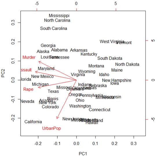
Red vectors are projections of the original
X-variables on the space of the first two principal components. We can see that
the first principal component Z1 mostly represents the combined
crime rate, and the second principal component Z2 mostly represents
the level of urbanization.
1.
K-means method
Now we use K-means clustering to find more
homogeneous groups among the states.
Let’s start with K=2 clusters. The 50 states are
partitioned into 2 groups, Cluster 1 with 21 and Cluster 2 with 29 states.
> KM2 = kmeans(X,2)
> KM2
K-means clustering with 2
clusters of sizes 21, 29
Cluster means:
Murder
Assault UrbanPop Rape
1 11.857143 255.0000
67.61905 28.11429
2 4.841379 109.7586 64.03448 16.24828
Clustering vector:
Alabama Alaska Arizona Arkansas California
1 1 1 1 1
Colorado Connecticut Delaware Florida Georgia
1 2 1 1 1
Hawaii Idaho Illinois Indiana Iowa
2 2 1 2 2
Kansas Kentucky Louisiana Maine Maryland
2 2 1 2 1
Massachusetts
Michigan Minnesota Mississippi Missouri
2 1 2 1 2
Montana Nebraska Nevada
New Hampshire New Jersey
2 2 1 2 2
New Mexico New York North Carolina North Dakota Ohio
1 1 1 2 2
Oklahoma Oregon Pennsylvania Rhode Island South Carolina
2 2 2 2 1
South Dakota Tennessee Texas Utah Vermont
2 1 1 2 2
Virginia Washington
West Virginia Wisconsin Wyoming
2 2 2 2 2
Within cluster sum of
squares by cluster:
[1] 41636.73 54762.30
(between_SS / total_SS = 72.9 %)
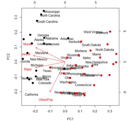
Let’s look at the position of these clusters on
our biplot. There is a discrepancy of scales in biplot, so I am using a
coefficient 3.5, to match points to state names.
> points(3.5*pc$x[,1],
3.5*pc$x[,2], col=KM2$cluster, lwd=5)
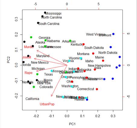
Use more clusters?
> KM5 = kmeans(X,5)
> points(3.5*pc$x[,1],
3.5*pc$x[,2], col=KM5$cluster, lwd=5)
2.
Hierarchical Clustering and Dendrogram
So, how many clusters should be used? We can
apply the hierarchical clustering algorithm, which does not require to
pre-specify the number of clusters.
> HC = hclust( dist(X),
method="complete" )
Here, “dist” stays for distance between
multivariate observations, and method can be “complete”, “single”, “average”,
“median”, etc. – it is a method of determining similarity with clusters and dissimilarity
between clusters.
We can see the dendrogram that this method has created.
> plot(HC)
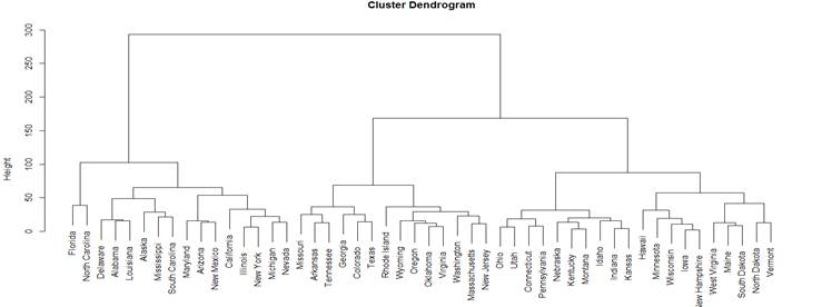
We then cut the tree at some level and create
clusters.
> cutree(HC,5)
Alabama Alaska Arizona Arkansas California
1 1 1 2 1
Colorado Connecticut Delaware Florida Georgia
2 3 1 4 2
Hawaii Idaho Illinois Indiana Iowa
5 3 1 3 5
Kansas Kentucky Louisiana Maine Maryland
3 3 1 5
1
Massachusetts Michigan Minnesota Mississippi Missouri
2 1 5 1 2
Montana Nebraska Nevada
New Hampshire New Jersey
3 3 1 5 2
New Mexico New York North Carolina North Dakota Ohio
1 1 4 5 3
Oklahoma Oregon Pennsylvania Rhode Island South Carolina
2 2 3 2 1
South Dakota Tennessee Texas Utah Vermont
5 2 2 3 5
Virginia Washington
West Virginia Wisconsin Wyoming
2 2 5 5 2
3.
College data - K-means method
Our task will be to cluster Colleges into more
homogeneous groups.
> attach(College); names(College)
[1] "Private" "Apps" "Accept" "Enroll" "Top10perc" "Top25perc" "F.Undergrad"
"P.Undergrad" "Outstate"
"Room.Board"
[11]
"Books"
"Personal"
"PhD"
"Terminal" "S.F.Ratio" "perc.alumni"
"Expend"
"Grad.Rate"
We need to create a matrix of numeric variables.
We’ve used this command to prepare data for LASSO.
> X = model.matrix( Private ~ .
+ as.numeric(Private), data=College )
> dim(X)
[1] 777 19
> head(X) Instead of printing the entire matrix, “head” only shows the first few
rows
(Intercept) Apps Accept Enroll Top10perc Top25perc F.Undergrad
P.Undergrad Outstate Room.Board Books Personal PhD
Abilene Christian University
1 1660 1232 721
23 52 2885 537
7440 3300 450
2200 70
Adelphi University
1 2186 1924 512
16 29 2683 1227
12280 6450 750
1500 29
Adrian College
1 1428 1097 336
22 50 1036 99
11250 3750 400
1165 53
Agnes Scott College
1 417 349
137 60 89 510 63
12960 5450 450
875 92
Alaska Pacific University
1 193 146
55 16 44 249 869
7560 4120 800
1500 76
Albertson College 1 587
479 158 38 62 678 41
13500 3335 500
675 67
Terminal S.F.Ratio perc.alumni Expend Grad.Rate as.numeric(Private)
Abilene Christian University
78 18.1 12
7041 60 2
Adelphi University
30 12.2 16
10527 56 2
Adrian College
66 12.9 30
8735 54 2
Agnes Scott College
97 7.7 37
19016 59 2
Alaska Pacific University
72 11.9 2
10922 15 2
Albertson College
73 9.4 11
9727 55 2
Now, let’s create K=5 clusters by the K-means
method. No new library is needed, this command comes with basic R.
> KM5 = kmeans( X, 5 )
> KM5
K-means clustering with 5 clusters of sizes 20, 113, 162, 431, 51
Cluster means:
(Intercept) Apps
Accept Enroll Top10perc
Top25perc F.Undergrad P.Undergrad
Outstate Room.Board Books
Personal PhD Terminal
1 1 9341.750 3606.2500 1321.9500 76.05000
91.70000 5283.200 427.2000 18119.750 6042.750 576.6000 1255.550 93.30000 96.80000
2 1 5012.602 3410.1150 1526.5310 21.56637
52.28319 8021.566 2111.3097
6709.283 3703.912 557.1416
1727.186 77.01770 83.65487
3 1 2566.364 1712.7901 521.5123
39.83333 68.96914 2067.241
282.4444 15732.512 5257.864
578.0926 1042.772 83.31481 90.24074
4 1 1140.610
869.9258 341.7007 21.40371
48.75638 1434.332 475.6450
9263.759 4110.290 530.1206
1299.220 65.03016 72.61717
5 1 13169.804 8994.7647
3438.1176 34.84314 67.15686
17836.020 3268.3529 8833.510
4374.353 593.0784 1813.784 85.54902 90.64706
S.F.Ratio perc.alumni Expend Grad.Rate as.numeric(Private)
1 6.61500 35.35000 32347.900 88.95000 2.000000
2 17.46903 14.02655
7067.257 54.91150 1.079646
3 11.43333 32.76543 13728.735 76.64198 1.993827
4 14.32343 21.36659
7677.035 63.13225 1.856148
5 15.99608 16.92157 10343.882 63.82353 1.117647
Clustering vector:
Abilene
Christian University
Adelphi University Adrian College
4
3 4
Agnes
Scott College Alaska
Pacific University
Albertson College
3
4 4
Albertus
Magnus College
Albion College Albright College
4 3 3
Alderson-Broaddus College Alfred
University
Allegheny College
4
3 3
<truncated>
Within cluster sum of squares by cluster:
[1] 2115931982 3262290091 3917614114 5524699694 5934672728
(between_SS / total_SS = 71.2 %)
Available components:
[1] "cluster"
"centers"
"totss"
"withinss"
"tot.withinss" "betweenss" "size" "iter" "ifault"
We can see the cluster assignment (truncated),
multivariate cluster means (centroids), within and between sums of squares as
measures of cluster purity. To explore the obtained clusters, we can plot some pairs
of variables along with the assigned clusters:
> par(mfrow=c(2,2))
> plot( Outstate, Top10perc, col=KM5$cluster
)
> plot( S.F.Ratio, PhD, col=KM5$cluster )
> plot( Apps, Enroll, col=KM5$cluster )
> plot( Room.Board, Private, col=KM5$cluster
)
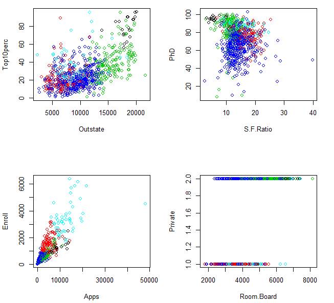
For example, we can see here that the green
cluster consists of rather expensive and relatively small private colleges with
a high percent of PhD degrees among faculty and small class sizes because of a
low student-to-faculty ratio.
4.
College data - Hierarchical Clustering
Without specifying the number K of clusters,
apply hierarchical clustering algorithm to the College data.
> HC = hclust( dist(X),
method="complete" )
Here, “dist” stays for distance between
multivariate observations, and method can be “complete”, “single”, “average”,
“median”, etc. – it is a method of determining similarity with clusters and
dissimilarity between clusters.
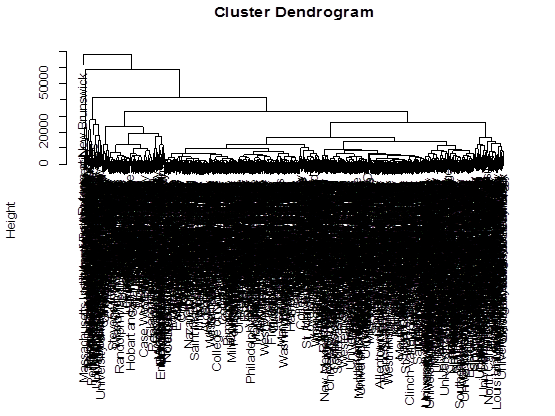
The full dendrogram with so many leafs would not
be legible.
> plot(HC)
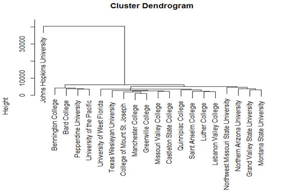
To illustrate the method, let’s take a small
random sample of colleges and cluster them hierarchically.
> Z = sample(n,20)
> Y = X[Z,]
> HCZ = hclust(
dist(Y), method="complete" )
> plot(HCZ)
We can choose where to “cut” this tree to create
clusters. For example, we let’s create 4 clusters.
> HC4 = cutree(HC, k = 4)
> HC4
Christian Brothers University Nazareth College of Rochester
1 1
Sweet Briar College Dartmouth College
1 2
Eckerd College Appalachian State University
1 3
< truncated >
So, we get assignments of colleges into
clusters.