APPLICATIONS

1. Matrix computation for Google’s PageRank algorithm

How to solve the matrix equation and obtain Google solution for the textbook example

(Elements of Statistical Learning, pp. 576-578)

> x=c(0,1,1,0,0,0,1,0,1,0,0,0,0,0,1,0)

> L = matrix(x,4,4) # Define a 4x4 matrix L showing linkage among web pages

> L # R reads a matrix column by column

[,1] [,2] [,3] [,4]

[1,] 0 0 1 0

[2,] 1 0 0 0

[3,] 1 1 0 1

[4,] 0 0 0 0

> e = matrix( rep(1,4), 4, 1 ) # Vector of 1s

> e

[,1]

[1,] 1

[2,] 1

[3,] 1

[4,] 1

> C = diag( colSums(L) ) # Diagonal matrix C showing the number

> C # of outgoing links from each web page

[,1] [,2] [,3] [,4]

[1,] 2 0 0 0 # Matrix multiplication is %*%

[2,] 0 1 0 0 # Inverse matrix is solve(C)

[3,] 0 0 1 0 # Transpose matrix is t(e)

[4,] 0 0 0 1

> A = 0.15*(e%*%t(e))/4 + 0.85*L%*%solve(C)

> A

[,1] [,2] [,3] [,4]

[1,] 0.0375 0.0375 0.8875 0.0375

[2,] 0.4625 0.0375 0.0375 0.0375

[3,] 0.4625 0.8875 0.0375 0.8875

[4,] 0.0375 0.0375 0.0375 0.0375

> eigen(A) # Computes eigenvalues and eigenvectors of A

$values

[1] 1.000000e+00+0.00e+00i -4.250000e-01+4.25e-01i

[3] -4.250000e-01-4.25e-01i 5.477659e-18+0.00e+00i

$vectors

[,1] [,2]

[1,] -0.64470397+0i 7.071068e-01+0.000000e+00i

[2,] -0.33889759+0i -3.535534e-01-3.535534e-01i

[3,] -0.68212419+0i -3.535534e-01+3.535534e-01i

[4,] -0.06489841+0i -2.175463e-17-4.017163e-18i

[,3] [,4]

[1,] 7.071068e-01+0.000000e+00i -9.941546e-16+0i

[2,] -3.535534e-01+3.535534e-01i -7.071068e-01+0i

[3,] -3.535534e-01-3.535534e-01i -1.968623e-16+0i

[4,] -2.175463e-17+4.017163e-18i 7.071068e-01+0i

> install.packages("expm”) # This package contains matrix powers

> library(expm) # “Exponentiation of a matrix”

> A100 = A%^%100 # Large power of matrix A

> A100 # (a simple but not an optimal method)

[,1] [,2] [,3] [,4]

[1,] 0.3725269 0.3725269 0.3725269 0.3725269

[2,] 0.1958239 0.1958239 0.1958239 0.1958239

[3,] 0.3941492 0.3941492 0.3941492 0.3941492

[4,] 0.0375000 0.0375000 0.0375000 0.0375000

# “Converged”! All columns are the same

> p = A100[,1] # Take one column of A¹⁰⁰

> p

[1] 0.3725269 0.1958239 0.3941492 0.0375000

> p=t(t(p)) # Now R understands it as a column

> p

[,1]

[1,] 0.3725269

[2,] 0.1958239

[3,] 0.3941492

[4,] 0.0375000

# Verify that it is a solution of p = Ap

> A%*%p

[,1]

[1,] 0.3725269

[2,] 0.1958239

[3,] 0.3941492

[4,] 0.0375000

# p is not properly normalized yet, we need e’p = N = 4

> t(e)%*%p # but we have the sum of p[i] = 1

[,1]

[1,] 1

> p*4 # This is the solution. Ranked by importance, we have

[,1] # web pages ordered as 3, 1, 2, 1

[1,] 1.4901074

[2,] 0.7832956

[3,] 1.5765969

[4,] 0.1500000

# Another way is by iterations (standard method of solving fixed-point equations):

> p = matrix(c(1,0,0,0),4,1) # The initial vector is kind of arbitrary

> p

[,1]

[1,] 1

[2,] 0

[3,] 0

[4,] 0

> for (n in (1:100)){ p = A%*%p } # Iterate p[next] = A*p[current]

> 4*p # Same result

[,1]

[1,] 1.4901074

[2,] 0.7832956

[3,] 1.5765969

[4,] 0.1500000

2. Spam detection

# The Spam data with description are in https://archive.ics.uci.edu/ml/datasets/Spambase

# We can also get its formatted version from a package “kernlab”

> library(kernlab)

> data(spam)

> dim(spam)

[1] 4601 58

> names(spam)

[1] "make" "address" "all" "num3d"

[5] "our" "over" "remove" "internet"

[9] "order" "mail" "receive" "will"

[13] "people" "report" "addresses" "free"

[17] "business" "email" "you" "credit"

[21] "your" "font" "num000" "money"

[25] "hp" "hpl" "george" "num650"

[29] "lab" "labs" "telnet" "num857"

[33] "data" "num415" "num85" "technology"

[37] "num1999" "parts" "pm" "direct"

[41] "cs" "meeting" "original" "project"

[45] "re" "edu" "table" "conference"

[49] "charSemicolon" "charRoundbracket" "charSquarebracket" "charExclamation"

[53] "charDollar" "charHash" "capitalAve" "capitalLong"

[57] "capitalTotal" "type"

> table(type)

type

nonspam spam

2788 1813

# LOGISTIC REGRESSION

> logreg = glm( type ~ ., data=spam, family = "binomial" )

> prob.spam = fitted.values(logreg)

> class.spam = ifelse( prob.spam > 0.5, "spam", "nonspam" )

> table(class.spam, type)

type

class.spam nonspam spam

nonspam 2666 194

spam 122 1619

> mean( type == class.spam )

[1] 0.9313193 # Correct classification rate = 93% (better be validated by CV)

# What are error rates among spam and benign emails?

> sum( type=="nonspam" & class.spam=="spam" ) / sum( type=="nonspam" )

[1] 0.04375897

> sum( type=="spam" & class.spam=="nonspam" ) / sum( type=="spam" )

[1] 0.107005

# Reducing the error rate for nonspam emails, with loss function L(1,0)=1, L(0,1)=10

> class.spam = ifelse( prob.spam > 10/11, "spam", "nonspam" )

> table(class.spam, type)

type

class.spam nonspam spam

nonspam 2759 674

spam 29 1139

> mean( type == class.spam )

[1] 0.8472071

> sum( type=="nonspam" & class.spam=="spam" ) / sum( type=="nonspam" )

[1] 0.01040172

> sum( type=="spam" & class.spam=="nonspam" ) / sum( type=="spam" )

[1] 0.3717595

# The overall error rate increased, and the error rate of misclassifying spam emails as nonspam increased substantially, but the error rate for benign emails is only 1% now.

# DECISION TREES

> tr = tree( type ~ ., data=spam )

> plot(tr); text(tr);

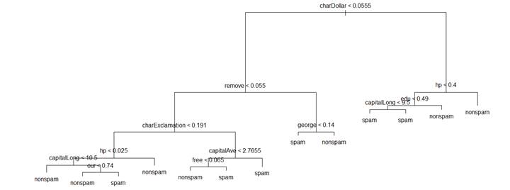
> summary(tr)

Misclassification error rate: 0.08259 = 380 / 4601

# Optimization – random forests

> library(randomForest)

> rf = randomForest( type ~ ., data=spam )

> varImpPlot(rf) # To see which variables are most significant in a tree based classification

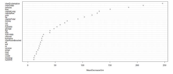
> rf

Number of trees: 500

No. of variables tried at each split: 7 # That’s approx. square root of the number of X-variables

OOB estimate of error rate: 4.52% # The lowest classification rate we could get so far

Confusion matrix:

nonspam spam class.error

nonspam 2710 78 0.02797704

spam 130 1683 0.07170436

# DISCRIMINANT ANALYSIS

> library(MASS)

> LDA = lda( type ~ ., data=spam, CV=TRUE )

> table( type, LDA$class )

type nonspam spam

nonspam 2656 132

spam 394 1419

> mean( type != LDA$class )

[1] 0.114323 # This error rate is higher

> QDA = qda( type ~ ., data=spam, CV=TRUE )

> table( type, QDA$class )

type nonspam spam

nonspam 2090 691

spam 87 1722

> mean( type != QDA$class )

[1] NA

> summary(QDA$class)

nonspam spam NA's

2177 2413 11 # There are missing values, predictions not computed by QDA

# We’ll remove these points

> mean( type != QDA$class, na.rm=TRUE )

[1] 0.1694989 # No improvement with QDA; linear models are ok

SUPPORT VECTOR MACHINES

> library(e1071)

> SVM = svm( type ~ ., data=spam, kernel="linear" )

> summary(SVM)

Number of Support Vectors: 940

( 456 484 ) # 940 support vectors (not cleanly classified) out of 4601 data points

> dim(spam)

[1] 4601 58

> class = predict(SVM)

> table(class,type)

type

class nonspam spam

nonspam 2663 185

spam 125 1628

> mean( class != type )

[1] 0.06737666 # Best rate so far?