Stat
622/422 (Dr. Baron) Advanced Biostatistics
First
steps in R. Variables, summary, folders, data sets
# Vectors and simple operations
> x <- c(1,3,5,6) # Create a vector (c means concatenate)
> x = c(1,3,5,6) # Another way to define a vector
> x
[1] 1 3 5 6
> x[2] # Get the 2nd element of vector x
[1] 3
> x[2:4]
# Get all elements of x
from the 2nd to the 4th
[1] 3 5 6
> x = rnorm(10000,2,100) # Generate a vector of 10,000 Normal random variables
# with mean 2 and st.
deviation 100
# Basic statistics
> mean(x)
[1] 2.379067
> sd(x)
[1] 100.0676
# Arithmetic operations
> x = c(1,3,5,7,0,-1)
> x
[1] 1 3
5 7 0 -1
> x^2
[1] 1 9 25 49
0 1
> sin(x)
[1] 0.8414710 0.1411200 -0.9589243 0.6569866
0.0000000 -0.8414710
> log(x)
[1] 0.000000 1.098612 1.609438 1.945910 -Inf
NaN
Warning message:
In log(x) : NaNs produced
# Define a matrix A based on a vector x
> A = matrix(x,2,3)
> A
[,1] [,2] [,3]
[1,] 1 5
0
[2,] 3 7
-1
# READING DATA FROM EXTERNAL FILES
# To point to the right folder, go "File" ->
"Change dir..." or use the setwd command
# Which folder is R pointed to right now?> getwd()[1] "C:/Users/baron/Documents" # Let's change the folder to the one where we have data. Notice slashes. > setwd("C:/Users/baron/Advanced Biostatistics/data")
# Use read.csv(“file.csv”) to read CSV viles,
read.table("file.txt") to read text files
# Rda and Rdata
files should be opened with load("file.rda")
> load("Heart.rda")
# Or, load data from a public domain
> Heart = read.csv("http://fs2.american.edu/baron/www/622/R/Heart.csv")
# Find out what variables are in the set
> dim(Heart)
[1] 303 15
> names
(Heart)
[1] "X"
"Age"
"Sex" "ChestPain" "RestBP" "Chol"
[7] "Fbs"
"RestECG" "MaxHR" "ExAng" "Oldpeak" "Slope"
[13] "Ca"
"Thal"
"AHD"
> summary
(Heart)
X Age Sex ChestPain
Min. :
1.0 Min. :29.00
Min. :0.0000 Length:303
1st Qu.: 76.5 1st Qu.:48.00 1st Qu.:0.0000 Class :character
Median :152.0 Median :56.00 Median :1.0000 Mode
:character
Mean :152.0
Mean :54.44 Mean
:0.6799
3rd Qu.:227.5 3rd Qu.:61.00 3rd Qu.:1.0000
Max. :303.0
Max. :77.00 Max.
:1.0000
RestBP Chol Fbs RestECG
Min. : 94.0
Min. :126.0 Min.
:0.0000 Min. :0.0000
1st Qu.:120.0 1st Qu.:211.0 1st Qu.:0.0000 1st Qu.:0.0000
Median :130.0 Median :241.0 Median :0.0000 Median :1.0000
Mean :131.7
Mean :246.7 Mean
:0.1485 Mean :0.9901
3rd Qu.:140.0 3rd Qu.:275.0 3rd Qu.:0.0000 3rd Qu.:2.0000
Max. :200.0
Max. :564.0 Max.
:1.0000 Max. :2.0000
MaxHR ExAng Oldpeak Slope Ca
Min. : 71.0
Min. :0.0000 Min.
:0.00 Min. :1.000
Min. :0.0000
1st Qu.:133.5 1st Qu.:0.0000 1st Qu.:0.00 1st Qu.:1.000 1st Qu.:0.0000
Median :153.0 Median :0.0000 Median :0.80 Median :2.000 Median :0.0000
Mean :149.6
Mean :0.3267 Mean
:1.04 Mean :1.601
Mean :0.6722
3rd Qu.:166.0 3rd Qu.:1.0000 3rd Qu.:1.60 3rd Qu.:2.000 3rd Qu.:1.0000
Max. :202.0
Max. :1.0000 Max.
:6.20 Max. :3.000
Max. :3.0000
NA's :4
Thal AHD
Length:303 Length:303
Class :character Class :character
Mode :character
Mode :character
# Look at the data as a spreadsheet
> fix(Heart)
# Refer to the particular variable in this dataset
with $ sign...
> Heart$Age
[1] 63 67 67 37 41 56 62
57 63 53 57 56 56 44 52 57 48 54 48 49 64 58 58
< truncated >
# or attach it the dataset that you plan to
work with...
> attach(Heart)
# Descriptive statistics: mean and the 5-number summary
> mean(Heart$Chol)
[1] 246.6931
> summary(Chol)
Min. 1st Qu. Median
Mean 3rd Qu. Max.
126.0 211.0
241.0 246.7 275.0
564.0
# PLOTS.
# Before you do anything with the data, look at them.
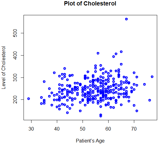
> plot(Age,Chol)

# Axis labels, graph title, color
> plot(Age, Chol, xlab="Patient’s Age", ylab="Level
of Cholesterol", main="Plot
of Cholesterol", col="blue",
lwd=3)
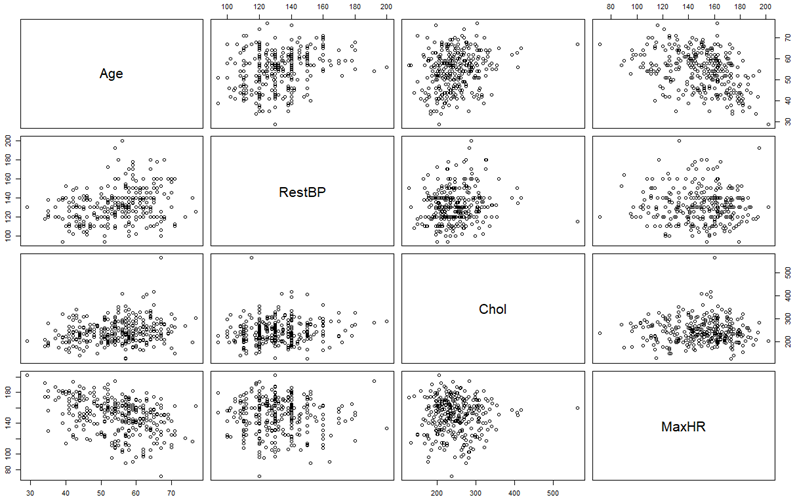
# SCATTERPLOT MATRIX ## Use it to plot more than 2 variables. # First, partition the graphing window into a matrix > par(mfrow=c(4,4)) # Then fill each non-diagonal space with the corresponding scatterplot > pairs(~Age+RestBP+Chol+MaxHR)
# Saving a graph in a file
> pdf("filename.pdf")
> plot(Chol, RestBP, col="blue")
> dev.off()
windows
2
# Finish and quit R
> q()